Index explained

27 jul 2023 - 8 minutes to read

Back-of-the-book index: includes names of people, places, events, and concepts selected by the indexer as being relevant and of interest to a possible reader of the book. (Wikipedia)

Database index: data structure that improves the speed of data retrieval operations on a database table. (Wikipedia)

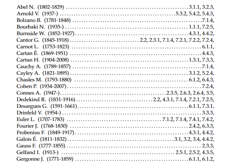
Introducing a blog post with two definitions of the same word is not accidental. Each of these provide a quick way to find a word or a term (or more broadly, a piece of data) using an normalized address, such as a page number in a book or the location of underligned data on a harddisk. In a purely academic way, just let us take the simplest indexing mechanism: when browsing an index to find a concept within a book, all references are arranged in alphanumeric order from top to bottom, from the left page to the right one (in Western literature).

Thus, readers can start their search from the first letter of their word, compare it to the sorted terms, start over with the second one, etc. until they find the correct term or the nearest related word. The result is then followed by a list of page numbers, in wich the author of the book has self-referenced the key concepts needed by the index search.

When talking about relational database system, entity (or object) related data are spread into columns owned by one or several tables. Looking at these data is similar to searching a word in a book: you need a search criteria (a surname, a date or even a join condition for example) and a access path (alphanumeric sort is the simplest one).

Reading a part of unindexed table content with SQL (like mentions in a book to a specific mathematician, for example) forces query executor to parse pages of the entire table (so called a full scan) and filter out all unneeded rows. This search is as effective as flipping through a book before coming across the information.

EXPLAIN statement can help us to determine which access method will be used by PostgreSQL to find mathematicians who belong to Gauss familly:

EXPLAIN (ANALYZE,BUFFERS) 
 SELECT firstname, lastname FROM mathematicians
  WHERE lastname = 'Gauss';

The result corresponds to the execution plan, also known as the query plan, built by a internal component, the planner, using available statistics, such as the number of known rows in the table, the presence of indexes, or the distribution of data according to their values (also called histogram). During this initial step, the planner can establish several plans and then choose the one with the lowest execution cost to ensure the overall processing time is as fast as possible.

                   QUERY PLAN 
-------------------------------------------------
Seq Scan on mathematicians  
 (cost=0.00..14.33 rows=1 width=18) 
 (actual time=0.188..0.189 rows=0 loops=1)
  Filter: ((lastname)::text = 'Gauss'::text)
  Rows Removed by Filter: 666
  Buffers: shared hit=6
Planning Time: 0.229 ms
Execution Time: 0.219 ms

The Seq Scan node confirms that the table was read sequentially and entirely, despite applying a filter. The ANALYZE option enriches the result at the cost of actually executing the query on the database relations (in this case, the mathematicians table). As a result, real search time and the number of returned and ignored rows are included in the output. The BUFFERS option indicates the number of blocks accessed, specifying whether they are read from shared memory (shared hit) or from the disk (read).

Let’s now observe the new execution plan when we add an index on the column lastname:

                          QUERY PLAN 
--------------------------------------------------------------
Index Scan using mathematicians_lastname_idx on mathematicians  
 (cost=0.28..8.29 rows=1 width=18)
 (actual time=0.043..0.046 rows=1 loops=1)
  Index Cond: ((lastname)::text = 'Gauss'::text)
  Buffers: shared hit=3
Planning Time: 0.176 ms
Execution Time: 0.081 ms

This time, the planner estimates a cost of 8.29 instead of 14.33 using the index on the search condition. We observe a change in the node considered by the planner: an Index Scan is now used to identify the unique entry for the value “Gauss” and retrieves the related information from the mathematicians table. As a result, the number of accessed blocks is reduced to 3, compared to 6 in the example without an index. The gain in execution time is significant: the query took 81 µs instead of 219.

However, this situation is not immutable, and depending on the value of the search, the best execution plan can vary. Let’s take the example of mathematicians from the Cartan family.

                          QUERY PLAN 
--------------------------------------------------------------
Bitmap Heap Scan on mathematicians
 (cost=4.29..8.85 rows=2 width=18) 
 (actual time=0.067..0.072 rows=2 loops=1)
  Recheck Cond: ((lastname)::text = 'Cartan'::text)
  Heap Blocks: exact=2
  Buffers: shared hit=4
  ->  Bitmap Index Scan on mathematicians_lastname_idx
       (cost=0.00..4.29 rows=2 width=0) 
       (actual time=0.051..0.051 rows=2 loops=1)
        Index Cond: ((lastname)::text = 'Cartan'::text)
        Buffers: shared read=2
Planning Time: 0.173 ms
Execution Time: 0.119 ms

We encounter another node related to the usage of an index, the Bitmap Heap Scan, and its Bitmap Index Scan. During its index traversal, the planner found two rows (rows=2) and stored their addresses in a memory array, also known as a bitmap. The retrieval of these rows involves random access, which can become costly for the planner.

For simple operations like equality, it is recommended to use a b-tree index, which is the default for CREATE INDEX. This index relies on an algorithm of the same name, which ensures the storage of key/value pairs within a balanced tree structure. The goal is to minimize the depth of the tree to reduce read costs.

A b-tree index is composed of:

• A meta block
• Intermediate blocks, including the root block
• Leaf blocks

You can inspect them using functions provided by the extensions pgstattuple and pageinspect, which allow you to unravel the index traversal performed by the executor phase.

 SELECT bt_page_stats.blkno, type, live_items
   FROM generate_series(1,
          pg_relpages('mathematicians_lastname_idx')::integer-1
        ) blkno,
LATERAL bt_page_stats('mathematicians_lastname_idx', blkno);

--  blkno | type | live_items 
-- -------+------+------------
--      1 | l    |        317
--      2 | l    |        319
--      3 | r    |          3
--      4 | l    |         32

The query is taken from french “PostgreSQL Architecture et notions avancées” by Guillaume Lelarge, edition D-BookeR.

The bt_page_stats method, associated with the index name and the block number, can be combined with the generate_series function to obtain one row per block belonging to the index, except for the meta block. We observe that block number 3 is the root (type=r) of our b-tree, the block from which the executor can perform successive comparisons until reaching the values of its search.

SELECT ctid, data, convert_from(decode(
         substring(replace(data, ' 00', ''), 4), 
       'hex'), 'utf8') as text
  FROM bt_page_items('mathematicians_lastname_idx', 3);

--   ctid   |                      data                       |     text     
-- ---------+-------------------------------------------------+--------------
--  (1,0)   |                                                 | 
--  (2,38)  | 0f 4b 6c 65 65 6e 65 00                         | Kleene
--  (4,116) | 1b 5a 61 72 61 6e 6b 69 65 77 69 63 7a 00 00 00 | Zarankiewicz

This root block lookup indicates that there are three branches (as indicated by the previous statistics with the value live_items of block number 3) containing the physical addresses of each leaf, also known as ctid. The data field varies depending on the type of indexed data and whether it is an index block or a table block. In this example, the text column indicates the lower bound (minus infinity) of each block. It is possible to obtain the boundaries of each leaf block with the following query:

SELECT blkno, min(text), max(text)
  FROM (
    SELECT blkno, convert_from(decode(
            substring(replace(data, ' 00', ''), 4), 
            'hex'), 'utf8') as text
      FROM (
        SELECT bt_page_stats.blkno 
          FROM generate_series(1,
                 pg_relpages('mathematicians_lastname_idx')::integer-1
               ) blkno,
        LATERAL bt_page_stats('mathematicians_lastname_idx', blkno)
          WHERE type = 'l'
      ) blkno,
   LATERAL bt_page_items('mathematicians_lastname_idx', blkno)
     WHERE length(data) > 0
  ) t GROUP BY blkno ORDER BY blkno;

--  blkno |     min      |     max      
-- -------+--------------+--------------
--      1 | Abbt         | Kleene
--      2 | Kleene       | Zarankiewicz
--      4 | Zarankiewicz | Zygmund

Returning to our previous search examples, both names “Gauss” and “Cartan” are classified between the letters A and K, which means they are located in block number 1 of the mathematicians_lastname_idx index. The traversal continues in this new leaf block, where the ctid addresses now correspond to the physical blocks of the mathematicians table.

SELECT *
  FROM (
    SELECT ctid, data, convert_from(decode(
             substring(replace(data, ' 00', ''), 4), 
           'hex'), 'utf8') as text
      FROM bt_page_items('mathematicians_lastname_idx', 1)
  ) t
 WHERE text IN ('Gauss', 'Cartan');

--   ctid   |          data           |  text  
-- ---------+-------------------------+--------
--  (3,8)   | 0f 43 61 72 74 61 6e 00 | Cartan
--  (4,8)   | 0f 43 61 72 74 61 6e 00 | Cartan
--  (1,102) | 0d 47 61 75 73 73 00 00 | Gauss

The results of the previous execution plans are now clear! As a reminder, we had an Index Scan node for the “Gauss” search and two Bitmap Heap/Index Scan nodes for the “Cartan” search.

The first search physically performs two reads in the index (blocks 3 and then 1) before reading the data block (1,102), making a total of three blocks, as mentionned by the execution plan (Buffers: shared hit=3).

The second search also involves two reads in the index but retrieves two distinct rows from two different locations in the table (addresses (3,8) and (4,8)), resulting in a total of four blocks, which aligns with the plan as well (Buffers: shared hit=4).

Of course, examining the contents of indexes is not necessary for performance analysis. Indexes are continuously maintained and balanced with every data modification to keep the physical addresses up to date and ensure optimized access with the lowest possible depth of traversal.

Adding an index should not be an automatic reflex. It is essential to consider the cardinality of the data in a column, which refers to the small proportion of data returned by each filter. In the case of the mathematicians table, a search based on LIKE or > conditions could easily scan all six blocks of the table (Seq Scan) because it is less costly than traversing multiple additional index blocks.

This article focused on the operation of the most common index, the b-tree. However, there are many other types of indexes that cater to various search and storage requirements!